Lesson

Guidelines for running effective Bayesian A/B tests

In this post, we describe the basic ideas behind Bayesian statistics and how they feed into business decisions you will need to make at the end of a test.

Ron Kenett

Professor Ron Kenett,

KPA Group

David Steinberg

Professor David Steinberg,

KPA Group

Please accept functional cookies to watch this video.

A/B testing is a great way to compare alternative experiences or possible modifications to your website or digital properties. By running the two experiences in parallel and deciding at random which visitors land on which version, you get an honest comparison of which one delivers better performance.

Once you get data insights from your test, you need reliable and informative ways to summarize them and reach conclusions. The Bayesian approach to doing statistics is a great way to accomplish this.

Here we describe the basic ideas behind Bayesian statistics and how they feed into the business decisions that you will need to make at the end of a test. We first present the approach to data insights analysis.

Then, we illustrate how this analysis leads to natural solutions for questions such as:

Which variant drives better results?

How much better are those results?

Can we be confident in our conclusion?

What if we want to test more than two variants?

What sample size is needed for a Bayesian A/B test?

Can a test be terminated early if results look clear?

What is Bayesian statistics?

Bayesian statistics is named after the Reverend Thomas Bayes who lived in Britain in the 18th century and was responsible for proving Bayes Theorem. The guiding principle in Bayesian statistics is that you can use the language of probability to describe anything that we don’t know and want to learn from data insights. As we will see, this is an ideal language for discussing many of the questions that are most important to business decisions.

When you run an A/B test, the primary goal is to discover which variant is most effective. To do so, you compare the results with the two methods. The Bayesian analysis begins by looking at the KPIs for each of the variants. The findings give us information about their value but always leave some uncertainty. We describe uncertainty using a probability distribution. We can simulate results from the distribution to understand how it looks.

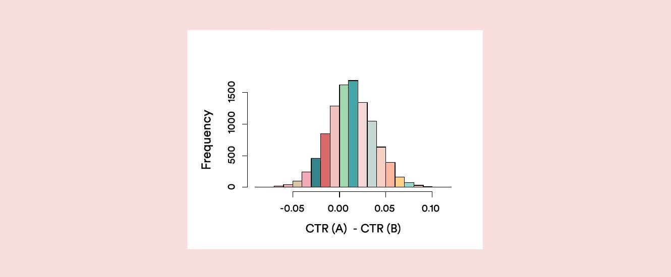
The histogram in Figure 1 is typical of what you might get from your analysis. It shows the statistical distribution of difference in click-through rate (CTR) between A and B. Most of the curve is to the right of 0, providing evidence that A has a higher CTR. The fraction of the curve to the right of 0 is a great summary of that evidence – it is called the Probability to Be Best (P2BB). In Figure 1, P2BB is 0.699, in favor of version A.

Graph of a distribution between frequency and CTR

If you have three or more variants, it is still easy to compute the probability of being best (P2BB), with probability split into three pieces, one for each variant.

How does Bayesian analysis work?

You need to start the Bayesian engine running with a prior probability distribution that reflects what you think about the KPI before seeing any data insights. The prior is then combined with your test data insights to obtain a posterior distribution for each variant. Figure 1 would be the posterior distribution for the difference between the A and B variants; this reflects the current view after having seen the data insights.

You need the prior to make things work, but when the volume of data insights is large — and that is almost always the case in A/B tests — the posterior is quickly dominated by them and virtually “forgets” the prior; so you don’t need to invest too much thought about how to choose the prior. It is possible to work with some standard choices for priors without affecting the analysis.

But can you really state a prior distribution and what you think in advance?

This has certainly been the source of friction between people in the different statistical camps, so it is helpful to contrast the Bayesian summary with the “classical,” Frequentist approach you might have studied in an introductory statistics course. In the classical approach, either A is better than B, B is better than A or they are identical. The question “what is the probability that A is better” is not part of the lexicon. You can’t give an answer, and in fact, you’re not even permitted to ask the question!

The classical paradigm does use probability, but only to describe the experimental data insights, not to summarize what you know about a KPI. That’s why you can’t make a summary like “the probability that B gives a positive uplift over A is 98%.

In most A/B tests, you’re getting lots and lots of data insights. Therefore, it no longer becomes very controversial, because whatever you put in to get the Bayesian engine going is essentially going to be washed out by that information, which is really going to be the component that dominates what you get in the end. And that’s why we think the Bayesian summaries are so much better suited for business decisions.

Check out this article for more on the different viewpoints when it comes to the Bayesian vs. Frequentist approach to A/B testing.

How should traffic be distributed between variations?

People who see option A should be, in some sense, as similar as possible to those who see option B. And it’s become well-established in the scientific literature, going back to work of the statistician Ronald Fisher about 100 years ago, that the best way to do that is to make sure that you choose the right traffic allocation.

So, think about the options that are on the table. If someone comes to your website, you must decide what landing page a visitor sees. You can control that by allocating one at random between the two groups. You must have an engine at your disposal — a framework that’s gonna let you make those random allocations. That will guarantee a fair comparison.

In order to validate the data insights that you’re capturing, you must ensure this random allocation occurs, as it establishes some causality on what is impacting user decisions. For instance, if you give the young people version A and the older people version B, and you see a difference, you will never know if it’s due to their age or the web page design. That’s called confounding.

What length of time is needed to run an A/B test?

In making these decisions, it is important to think about “what might go wrong” with the testing engine. You want your test to be sensitive to possible bugs. Often bugs are related to failures of the random allocation over time so that natural time trends in your KPIs bias the results. If there are weekly trends in your data insights, then you need to run an A/B test for two weeks to make sure that the engine is successfully handling them. If there are diurnal trends (but not weekly), you can afford to run shorter experiments. There may also be special events that suddenly increase or decrease the number of visitors to your site, or change the composition of visitors, affecting the performance of an experience. You may want to hold off on making any decisions until you see whether such issues have an impact on your results.

The considerations noted above will suggest a minimum time frame for running your experiment that ensures representative coverage in the A/B test of typical future site visitors. Often, these will dictate the length of time for the test.

How large a sample size is needed for a Bayesian test?

The sample size paradigm for Bayesian testing asks how narrow you want your final probability functions to be. You will probably want to focus on the probability function for the difference in KPIs between the two variants, as shown in Figure 1. And you will already have an idea what sort of difference could be important for your business; that gives a guideline for how narrow you want the function to be — the tighter the interval, the more you know.

It’s important to note that you can have a tight interval, but if the people who looked at the website and were part of the randomization subgroup, then whatever you’re going to get will not apply to the general group. So you really should work on both fronts. One is, how much information do you have? The tighter the interval, the more informative it is. But also how generalizable is the information that you provide?

Both of these aspects are important and can be the driver in dictating how large an experiment has to be. A website that has very heavy volume may quickly get to the needed sample size but without being able to see the full representative picture of all the visitors. And this can happen the other way around too, so that by the time you get the sample size you need, you’ve already gone through several time cycles; you must see how both of these work out and balance against one another.

You will need to provide information on likely values for the KPIs. Often one of the versions is already running, so you can use historical data insights for this purpose. For new versions, you will need to think about what effect they might have. If the test includes multiple versions, the same ideas apply, and the same inputs are needed.

The basic inputs needed to compute a sample size depend on the nature of the KPI:

For binary KPIs like CTR or installation rate, all you need are the expected rates for each version

If you are looking at purely continuous KPIs like revenue per conversion, you will need to supply an estimate of both the typical conversion size and the variation in size among those who do convert

For a “mixed” KPI like revenue per visitor, you will need the average, variation and an estimate of the fraction who will convert.

There are straightforward formulas you can use to determine the sample size as well as helpful A/B test sample size calculators. The considerations noted above will suggest a minimum time frame for running your experiment that ensures representative coverage in the A/B test of typical future site visitors. Often, these will dictate the length of time for the test.

What if there are more than two versions in the test?

The same sample size formulas are relevant, but here we distinguish between two goals: (1) finding the best and (2) showing that the standard version is not the best.

What is different about the second goal?

Suppose you have two new versions that you want to compare to the standard. Your best guess gives almost the same expected KPI to each of the new versions, with both of them improving over the standard. With very similar KPI’s, you will need a large sample to know which of the two new versions is better than the other. But if you expect both to be better than the standard, you can “rule out” the standard version with a much smaller test.

To further illustrate the idea:

The current experience is getting a CTR of 1%. A new version is proposed with the expectation that it will increase the CTR to 1.2%. The expected difference is 0.2%, so you need an A/B test that will tell you what is the true difference to a higher resolution. A good rule of thumb is to aim for a resolution that concentrates 95% of the Posterior Distribution in an interval that is the size of the expected difference.

In this example, that means narrowing down the difference so that you are 95% certain about an interval of length 0.002. To achieve this level of accuracy, you will need a sample of 83,575 visitors to both pages. What if even a 10% improvement in CTR to 1.1% is critical? Then you would need to know the difference up to, at most, 0.1%. That will require a sample size of 319,290 for each version.

Now let’s look at an example involving revenue per visitor:

A common scenario (often referred to as the Pareto principle)is that most visitors don’t provide any revenue and, among those who do, a small number of “big fish” pull up the average, and also the standard deviation.

The current landing page has a conversion rate of 1%; on average, converters spend $20; the standard deviation in the purchases of converters is $25. That means the average revenue per visitor is $0.20. Marketing thinks that the new version will bring in more purchasers, upping the conversion rate to 1.2%, but will decrease the proportion of “big fish,” so that the average conversion drops to $19 and the standard deviation to $22.

That translates to an average revenue of $0.228, an expected improvement of $0.028 per visitor. The A/B test will need to be large enough to narrow down the 95% credible interval for the difference in average revenue to no more than the expected difference, i.e. to $0.028. We will need 397,830 visitors to each experience to achieve that level of accuracy.

What if we want a stronger guarantee that we will find the important difference?

We advised above setting the sample size to control the width of the 95% credible interval. It is easy to reduce the chance of missing a valuable change by insisting on a higher level of probability, say 98% or 99%, but at the expense of increasing the sample size.

Can you stop a test early?

The probability that A is better (or worse) than B provides a natural metric to follow as the test progresses. And a strong signal from the P2BB statistic can be used to guide early stopping. However, early stopping needs to be done with caution.

First, the Bayesian summary is not completely immune to peeking. The P2BB will drift up and down during an experiment. This is especially true if there is no difference in performance between the variants, as in A/A testing. In that case, you will see that the P2BB increases and decreases as you collect more data insights. The fact that it crossed a threshold (like 95%) at some point during the test is not a guarantee that it would remain above the threshold if you wait until the planned termination time.

Second, it is always risky to stop before observing at least one full time cycle. Version B might be better for visitors at the start of the cycle, but worse for those later in the cycle. If you stop before the end of a full cycle, your results may be biased.

If you want to stop early, think about using stricter criteria for an early stopping point. For example, if you see that the probability becomes extreme (say above 0.999 or below 0.001), you can feel safe in stopping and making a decision. If there really is a difference between A and B, you can still expect to reach those thresholds relatively quickly.

Finally, we also reiterate the importance of waiting for time trends to reveal themselves in your test. You don’t want to decide on the basis of a short time window only to find that the results are very different later in the day or week — suppose weekday visitors respond better to A than B, but that trend flips on the weekend. Making a decision Wednesday from an experiment that began on Tuesday might lead to a bad decision.