The bayesian approach to A/B testing

The applications of A/B testing are age-old and spread across industries, from medical drug testing to optimizing experiences within e-commerce. But as the tools used to make informed decisions based on collected data insights continue to evolve, so too has the best approach. 

Once universally accepted, the Frequentist Approach to statistical inference in A/B testing scenarios is now being replaced by a new gold standard. Also based on the foundation of Hypothesis Testing, the Bayesian Approach is known for its less restrictive, highly intuitive and more reliable nature. While Mastercard Dynamic Yield has already written about the matter, my goal is to dive into the numbers behind the Bayesians school of thought, performing the appropriate derivations where necessary. 

In a Bayesian approach, everything is a random variable and by extension, has probability distribution and parameters. 

In Frequentist, if we want to model the click-through rate of a group, we try to find its mean and its variance, which act as the parameters. And to find these parameters, we collect sample data insights, write down likelihood and then maximize it with respect to the parameters. We go on to build confidence intervals around this Maximum Likelihood click-through rate to quantify the uncertainty around where the real mean would lie. 

In Bayesian, the real mean is a distribution but the observations are fixed, which models real life decision-making much better. To be more precise, in the case of a Bernoulli distribution, the probability mass function (pmf) is defined as:

With π being the probability for clicking. 

Here, according to the Bayesian approach, π should also have a distribution of its own, its own parameters, etc. 

To calculate the mean click-through rate, similar to the Maximum Likelihood mean value in a traditional A/B test, we try to solve for the value π in the below equation: 

Where X = the observed data insights. 

We apply the good old Bayesian conditional probability equation:

Here, p(X) can be treated as a normalizing constant, given its independence from π.

Therefore: 

p(π) = probability of click before the experiment began – the prior
p(X|π) = observed data samples – the likelihood
p(π|X) = probability of click after observing the sample – the posterior

We can calculate the p(X) value (probability of click-through) given the observed sample data insights is a product of prior and likelihood. Here, prior probability is the probability to click on a variation before any sample data insights are collected (this would be the historical average of an experiment or in the absence of any data, can be equated to a uniform distribution), and likelihood, on the other hand, the probability distribution of the collected sample data insights.

To solve this equation, we exploit a concept called Conjugate Prior. In Bayesian probability theory, if the posterior distribution has the same probability distribution as the prior probability distribution given a likelihood function, then the prior and posterior are called conjugate distributions. The prior is called a conjugate prior for the likelihood function.

In our case, if the likelihood function is Bernoulli distributed, choosing a beta prior over the mean will ensure the posterior distribution is also beta distributed. In essence, the beta distribution is a conjugate prior for the likelihood that is Bernoulli distributed! 

Let’s see how exploiting this concept helps us solve the posterior probability for both continuous and binary variables.

As we are dealing with a Bernoulli distribution, we only have to deal with one random variable (π). Assuming our likelihood function follows a prior-beta distribution: 

Also assuming the experiment begins with no prejudice, a beta distribution for the prior with α=1; β=1 would be a good starting point as beta (1,1) is a uniform distribution: 

Grouping the similar terms together: 

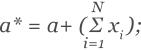
We can see the posterior is simply a beta distribution of the form:

Where:

Which is the same as our prior probability distribution:

Thus, confirming the conjugate priors concept for binary outcomes.

To solve for a posterior probability for binary outcomes, the blueprint would be:

1. π ~ Beta (1,1): assume the prior distribution is uniform
2. Sample x1
3. π ~ Beta (1+x1 ,1+1- x1): update the beta distribution to account for the sample observed data
4. Sample x2
5. π ~ Beta (1+x2 ,1+2- x2)
6. Repeat from Step 2

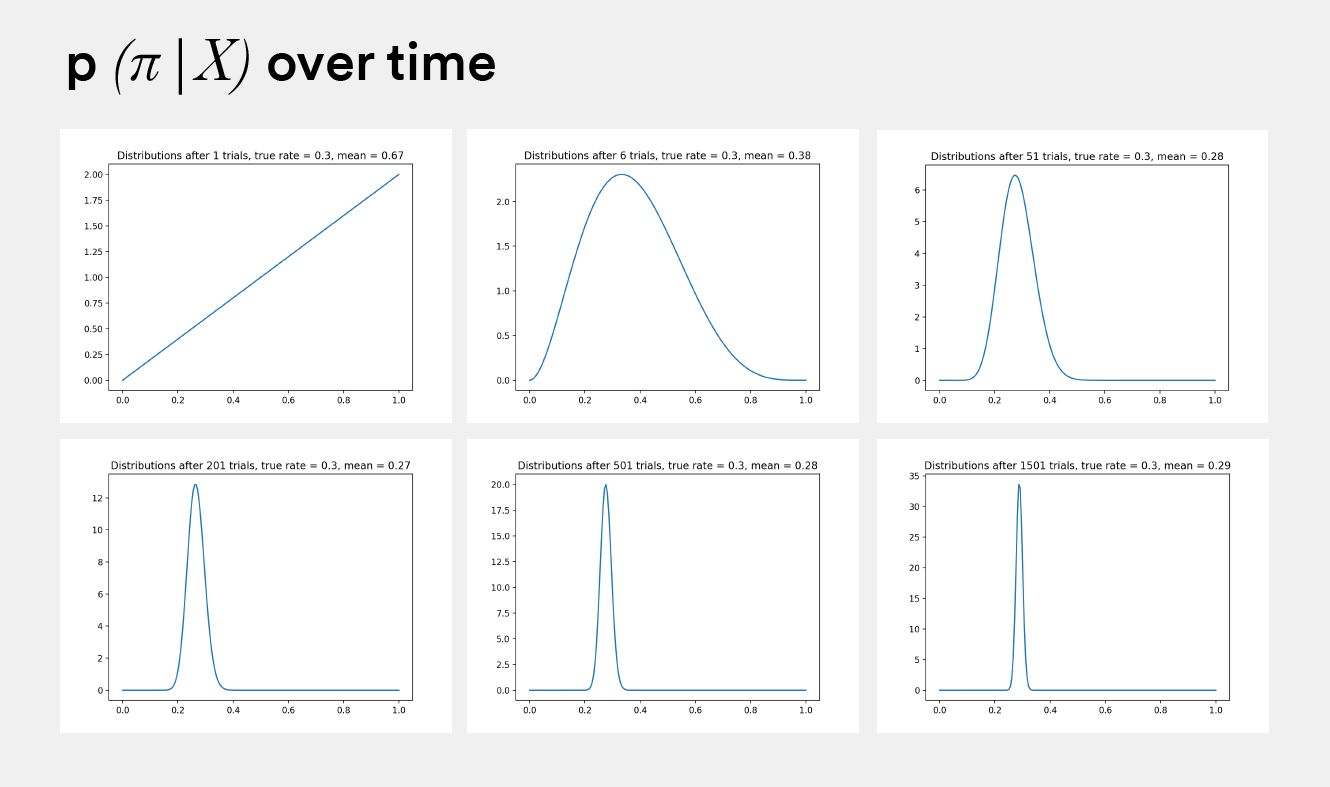
In the end, we reach a beta distribution that progresses from a uniform distribution to a skinny, normal distribution.

The following code, implemented in Python, will allow you to more easily visualize the progression, effectively demonstrating how the Bayesian probability changes over time as the number of samples increase

The progression of π over time can be seen as:

As we are dealing with a Bernoulli distribution, we only have to deal with one random variable (π). Assuming our likelihood function follows a prior-beta distribution:
 

For optimizing metrics that are discrete, such as the number of purchases, pageviews, and so on, we work with a gamma prior and Poisson likelihood. Again, resulting in a gamma posterior.

Imagine you are at a casino and out of two slot machines, you pick one and win 3/3 times played. What would your next move be? Would you continue to play with the machine that has proven to win or try the other one? 

This situation precisely sums up the explore-exploit dilemma — the choice between gathering more data insights and maximizing returns, which we already described closely applies to A/B testing. 

In a traditional A/B test, because you assign a percentage of the traffic, there is no option to exploit the data insights, i.e. incrementally assign more traffic to the winning variation. 

Let’s see how this is accomplished in a Bayesian setting. 

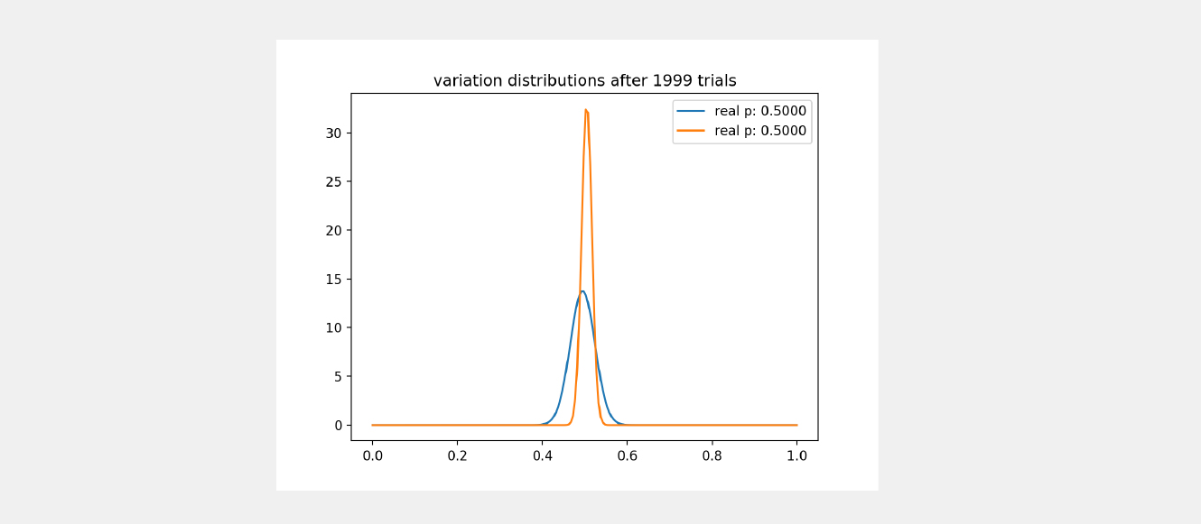
In short, sampling completely takes care of the explore-exploit dilemma for us in a Bayesian test. Say you have distributed traffic randomly between two variations (blue and orange) and reached the following posterior probability distribution for both: 

As can be seen, the orange variation is clearly sampled much more than the blue variation. And how do we acknowledge this? The variance! We saw earlier that a posterior probability gets skinnier with more sample data insights, so given that the blue variation is still chubbier, we can conclude it is not sampled enough. 

At this point, if we decide to randomly sample two points, one from each variation, and compare them both, what are the chances the orange variation would be higher? 

1. If the sample from the blue variation comes from the right half of the plot, then it would have better probability to be higher 

1. If the sample from the blue variation comes from the left half of the plot, then it would likely be lower than the orange variation 

What happens if we decide on the variation to show next based on which has the higher value in this random sampling? 

→ If the blue variation wins, it would then be shown next to the audience, furthering its sampling while also narrowing around a fixed probability for its true mean value. Here, we see two additional possibilities: 

• Its final probability > orange variation’s probability: If the sampling is continued, the blue variation would continue winning 

• Its final probability < orange variation’s probability: Orange variation would be sampled more and continue being shown 

→ If the blue variation loses, the orange variation is shown 

Therefore, sampling takes care of the explore-exploit dilemma for us, always making the best decision on our behalf. 

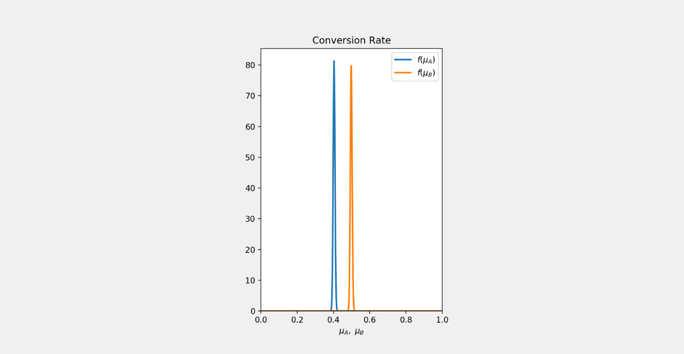
Once the posterior distributions are mapped for the variations, to conclude a winner, you sample a large amount of observations. Hypothetically, let’s say you sample 1000 times from two variations and 999 times out of 1,000 you see the orange variation having higher probability: 

The probability that variation orange is better than variation blue will be (999/1000) * 100, which is 99.9%. 

At Mastercard Dynamic Yield, we sample 300,000 times from every variation to calculate the Probability to Be Best (P2BB). 

When running a traditional A/B test where one variation is clearly outperforming another, the losing variation is still shown to a large audience until the statistical significance is reached. While allowing for confident winner-declaration, the time spent waiting can result in a loss of potential business. 

In an ideal world, you should be able to drop traffic to the losing variation and maximize returns with the winning variation. To provide the losing variation an opportunity to take the lead, we assign a bare minimum percentage of the traffic to it (called epsilon) and exploit the winning variation. Thus, the term ‘explore vs. exploit’ (also called ‘epsilon-greedy’ in some circles) has come to be, which addresses how much time is “wasted” on learning as opposed to taking advantage of what is already learned. This feature is nearly impossible in a traditional A/B test, unless you are hell-bent on producing false positives.

Recapping everything that has been laid out so far: 

• Bayesian A/B testing converges quicker than a traditional A/B test with smaller sample audience data insights because of its less restrictive assumptions 

• Achieving significance is ‘incremental’ by nature in Bayesian A/B testing. You can check the values at any time and decide to discontinue the experiment 

• Negligible chance of a false positive error 

• Explore-exploit strategy in Bayesian testing does not leave money on the table 

To conclude, the industry is moving toward the Bayesian framework as it is a simpler, less restrictive, highly intuitive and more reliable approach to A/B testing. In fact, Mastercard Dynamic Yield has made the move to a Bayesian statistical engine, not only for binary objectives such as goal conversion rate and CTR but also for non-binary objectives such as revenue per user. 

If you’d like to learn more about the issues presented in the Frequentist Approach, check out this blog post.